import numpy as np
from matplotlib import pyplot as plt
from ichor.core.models.kernels.distance import Distance
def se_kernel(a, b, sigma,l):
"""definition of SE kernel with lengthscale and variance"""
dist2 = Distance.squared_euclidean_distance(a, b)
return sigma**2*np.exp(-dist2/(2*l**2))
train_x = np.linspace(0, 6, 25).reshape(-1,1)
train_y = np.sin(train_x)
test_x = np.linspace(0, 6, 50).reshape(-1,1)
test_x_true = np.sin(test_x)
ntrain = train_x.shape[0]
mu = 0.0
LENGTHSCALE = 2.0
OUTPUTSCALE = 1.0
NOISE = 1e-12 * np.eye(ntrain)
K = se_kernel(train_x, train_x, OUTPUTSCALE, LENGTHSCALE) + NOISE # n_train x n_train with noise on diagonal
K_s = se_kernel(test_x, train_x, OUTPUTSCALE, LENGTHSCALE) # ntest x n_train
K_ss = se_kernel(test_x, test_x, OUTPUTSCALE, LENGTHSCALE) # n_test x n_test
L = np.linalg.cholesky(K)
alpha = np.linalg.solve(L.T, np.linalg.solve(L, train_y)) # weights
v = np.linalg.solve(L, K_s.T) # temp vector to calculate variance
predictions = (mu + np.matmul(K_s, alpha)).flatten()
posterior_covariance = K_ss - np.dot(v.T, v)
var = np.diag(posterior_covariance)
stdv = np.sqrt(var)
errors = test_x_true.flatten() - predictions
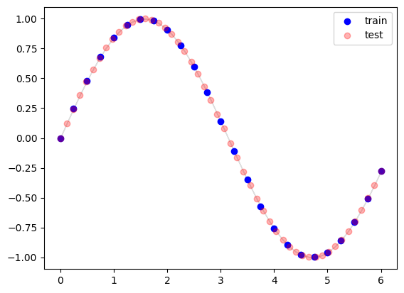
plt.gca().fill_between(test_x.flatten(), predictions-2*stdv, predictions+2*stdv, color="#dddddd") # 2 sigma confidence interval
# plt.plot(train_x, train_y)
plt.scatter(train_x, train_y, color="b", label="train")
plt.scatter(test_x, predictions, color="r", label="test", alpha=0.3)
plt.legend()
plt.show()